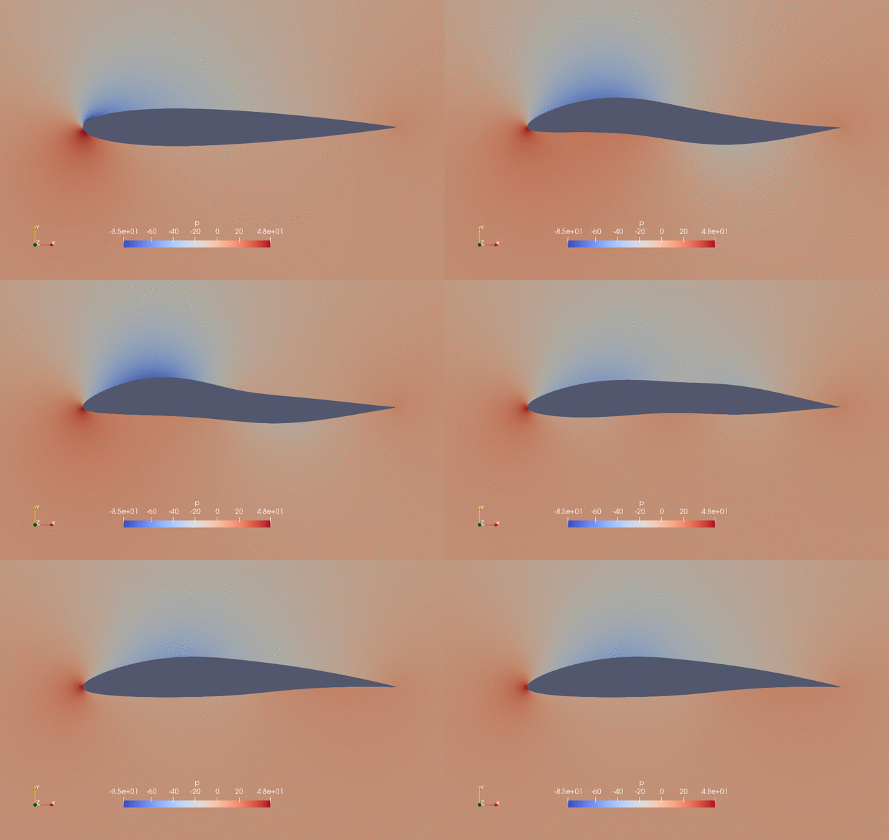
Fig. 1. Pressure and shape evaluation during the optimization process
Check optimization output file opt_SLSQP.txt
Once optimization is done, first check “opt_SLSQP.txt” in tutorials-master/NACA0012_Airfoil/incompressible. “opt_SLSQP.txt” contains the variation of objective function with respect to the optimization iteration:
       ---------------------------------------------------------------------------
         START OF THE SEQUENTIAL LEAST SQUARES PROGRAMMING ALGORIT
       ---------------------------------------------------------------------------

         PARAMETERS:
            ACC =   0.1000D-06
            MAXITER = 50
            IPRINT =   1
    IOUT =   6

         ITER =    1     OBJ =  0.20031286E-01
         ITER =    2     OBJ =  0.19239441E-01
         ITER =    3     OBJ =  0.19095023E-01
         ITER =    4     OBJ =  0.19040727E-01
         ITER =    5     OBJ =  0.19025003E-01
         .....
         .....
         .....
         ITER =   45     OBJ =  0.17376811E-01
         ITER =   46     OBJ =  0.17376810E-01
         ITER =   47     OBJ =  0.17376808E-01
         ITER =   48     OBJ =  0.17376811E-01
         ITER =   49     OBJ =  0.17376808E-01
         ITER =   50     OBJ =  0.17376808E-01
            NUMBER OF FUNC-CALLS:  NFUNC = 170
            NUMBER OF GRAD-CALLS:  NGRAD =  51
In this case, we use the SLSQP optimizer that prints objective function value from the 1st iteration. To find the objective for the 0th iteration (baseline design), you need to go back to “logOpt.txt” (see more detailed explanation of this file from this page):
+--------------------------------------------------------------------------+
|                  Evaluating Objective Functions 000                      |
+--------------------------------------------------------------------------+
Design Variables:
OrderedDict([('alpha', array([5.139186])), ('shapey', array([0., 0., 0., 0., 0., 0., 0., 0., 0., 0., 0., 0., 0., 0., 0., 0., 0.,
       0., 0., 0.]))])
....
....
....
Objective Functions:
{'DVCon1_volume_constraint_0': 1.0000000000000018, 'DVCon1_thickness_constraints_0': array([1.0000000000000102, 0.9999999999999997, 1.0000000000000004,
       1.0000000000000002, 1.                , 1.0000000000000002,
       0.9999999999999994, 1.0000000000000002, 0.9999999999999998,
       1.0000000000000033, 1.0000000000000056, 0.9999999999999996,
       0.9999999999999999, 1.0000000000000002, 1.0000000000000002,
       1.0000000000000002, 0.9999999999999998, 1.0000000000000002,
       0.9999999999999998, 1.0000000000000007]), 'CD': 0.020820258191996517, 'CL': 0.4999999575481259, 'fail': False}
Flow Runtime: 2.62659
The objective (CD) is 0.020820258 for the baseline design and drops to 0.017376808 for the 50th optimization iteration with a drag reduction of 16.5%.
Visualize the flow fields using Paraview
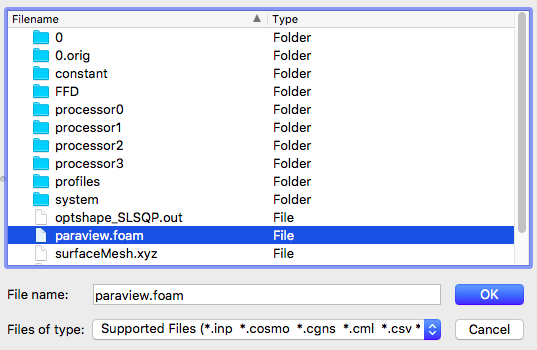
Next, we can use Paraview to visualize the flow fields. Download the Paraview binaries from here. They are ready to use for Windows, Linux, and MacOS. Once installed, open the Paraview app and click “File->Open…” from the top menu. In the pop-up window, navigate to tutorials-master/NACA0012_Airfoil/incompressible, select the paraview.foam file, and click “OK”.

Fig. 2. Open the paraview.foam file
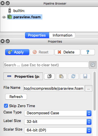
Then at the left panel, select “Decomposed Case” for “Case Type”.

Fig. 3. Select Case Type
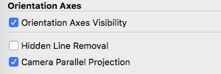
Next, scroll down at the left panel and check “Camera Parallel Projection”.

Fig. 4. Check Camera Parallel Projection
Now, click “Apply” at the left panel to load the flow fields. By default, the pressure field (p) will be load, but you can choose other flow variables to load at the top panel. Also, the “Surface” representation will be used by default, you can change it to “Surface With Edges” to visualize the mesh.

Fig. 5. Change variable to load and surface representation
Finally, you can hit the play button at the top panel to play a movie of evolution of pressure field and shape during the optimization (see the movie at the beginning of this page).

Fig. 6. Hit play to visualize a movie of optimization process
Refer to the Paraview User Guide for more advanced usage.
In the next page, we will elaborate on optimization run scripts and configuration files.