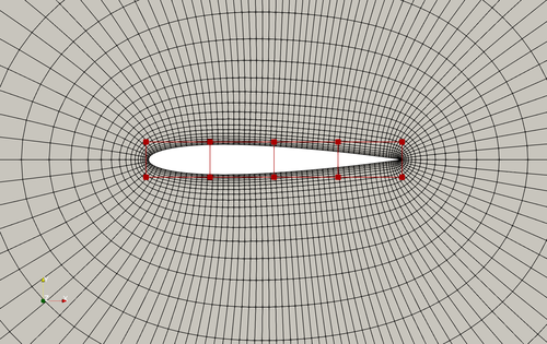
The following is a multipoint aerodynamic shape optimization case for the NACA0012 airfoil at low speed. We optimize the weighted drag coefficient considering three different flight conditions, i.e., CL=0.3, 0.7, and 0.5 (nominal). The weight of these three conditions are 0.25, 0.25, and 0.5, respectively.
Case: Airfoil aerodynamic optimization
Geometry: NACA0012
Objective function: Weighted drag coefficient (CD)
Lift coefficient (CL): 0.3, 0.7, and 0.5 (nominal)
Weights: 0.25, 0.25, 0.5 (nominal)
Design variables: 20 free-form deformation (FFD) points moving in the y direction, three angle of attacks
Constraints: Symmetry, volume, thickness, and lift constraints (total number: 34)
Mach number: 0.02941 (10 m/s)
Reynolds number: 0.6667 million
Mesh cells: ~4,000
Solver: DASimpleFoam

Fig. 1. Mesh and FFD points for the NACA0012 airfoil
The runScript.py is based on the one used in the NACA0012 low speed case with the following modifications:
-
In the global parameters, we define the number of multipoint configurations
nMultiPoints = 3, and set far field boundary conditions and flight conditios for all the three configurations.MPWeights,U0,alpha0, andCL_targetare the weights, far field velocity, angle of attack, and target lift coefficient for the three configurations. Note that we set the nominal conditionsCL_target = 0.5as the last element in the list such that the intermdiate flow fields will be saved for this condition, which facilitates the post-processing using Paraview.# global parameters nMultiPoints = 3 MPWeights = [0.25, 0.25, 0.5] U0 = [10.0, 10.0, 10.0] # we use the first U0 as reference velocity to normalize CD and CL URef = U0[0] CL_target = [0.3, 0.7, 0.5] alpha0 = [3.008097, 7.622412, 5.139186] p0 = 0.0 nuTilda0 = 4.5e-5 A0 = 0.1 -
In
daOptionswe set"multiPoint": Trueto activatve the multipoint optimization mode, and set"nMultiPoints": nMultiPoints. -
In the design variable setup section, we add three angle of attack design variables, each for one flight condition. We also append
mp0_,mp1_, andmp2_to the name of the angle of attack variable. Note: we provide a dummy function (dummyFunc) for alpha variable. This is because we will use a functionsetMultiPointConditionto change the angle of attack later inrunScript.py, so there is no need to provide an alpha function forDVGeo.addGeoDVGlobalhere.for i in range(nMultiPoints): DVGeo.addGeoDVGlobal("mp%d_alpha" % i, alpha0[i], dummyFunc, lower=0.0, upper=10.0, scale=1.0) # add alpha for designVar daOptions["designVar"]["mp%d_alpha" % i] = { "designVarType": "AOA", "patch": "inout", "flowAxis": "x", "normalAxis": "y", } -
In the optFuncs setup section. We provide a
setMultiPointConditionfunction to set flow boundary conditions for the three flight configurations. HeresetMultiPointConditionuses the design variable dictionaryxDVand the multipointindexas the input, and it implements a general method to change the boundary conditions. For this case, we first extract the alpha value fromxDV, compute the far field velocity components, replace theprimalBCkey in DAOption and update its value in DASolver (DASolver.updateDAOption()).def setMultiPointCondition(xDV, index): aoa = xDV["mp%d_alpha" % index].real * np.pi / 180.0 inletU = [float(U0[index] * np.cos(aoa)), float(U0[index] * np.sin(aoa)), 0] DASolver.setOption("primalBC", {"U0": {"variable": "U", "patch": "inout", "value": inletU}}) DASolver.updateDAOption() return -
Next, we define a function (
setMultiPointObjFuncs) to combine the objective function values. This function will be used in optFuncs.calcObjFuncValuesMP.def setMultiPointObjFuncs(funcs, funcsMP, index): for key in funcs: if "fail" in key: pass elif "DVCon" in key: funcsMP[key] = funcs[key] elif "CD" in key: try: funcsMP["obj"] += funcs[key] * MPWeights[index] except Exception: funcsMP["obj"] = 0.0 funcsMP["obj"] += funcs[key] * MPWeights[index] elif "CL" in key: funcsMP["mp%d_CL" % index] = funcs[key] returnIn optFuncs.calcObjFuncValuesMP, we loop over all the flight conditions and call
DASolver()to solve the primal and compute the objective dictfuncs. Then we callsetMultiPointObjFuncs, which takesfuncsand multipointindexas input, and outputs the dictfuncsMP, whereMPmeans multipoint.funcscontains the objective and constraint function values and afailflag. Here we create aobjkey by combiningCDcomputed from each flight condition. An example is as follows.funcs = {"CD": 0.01, "CL": 0.3, "DVCon_0": 1.0, "fail": False} # flight condition 0 funcs = {"CD": 0.03, "CL": 0.7, "DVCon_0": 1.0, "fail": False} # flight condition 1 funcs = {"CD": 0.02, "CL": 0.5, "DVCon_0": 1.0, "fail": False} # flight condition 2 # weights for the three flight conditions are 0.25, 0.25 and 0.5 funcsMP = {"obj": 0.02, "mp0_CL": 0.3, "mp1_CL": 0.7, "mp2_CL": 0.5, "DVCon_0": 1.0, "fail": False} # funcs for multipointNote that we do not combine CL, instead we keep all the lift coefficients by appending
mp0_,mp1_, andmp2_to the objective function names. This will allow us to set lift constraints for all flight conditions (seeoptProb.addConinrunScript.py). Also note that the geometry constraints (DVCon) are same for all three flight conditions, therefore there is no need to do weighting or appending any prefix names toDVCon. -
In addition, we define a function
setMultiPointObjFuncsSensto combine the objective function derivatives. This function will be used in optFuncs.calcObjFuncSensMP. In optFuncs.calcObjFuncSensMP, we loop over all the flight conditions and callDASolver.solveAdjoint()to solve the adjoint and compute the objective derivative dictfuncsSens. ThensetMultiPointObjFuncsSenstakes design variable dictxDVs, the mulitpoint objective value dictfuncsMP, objective derivative dictfuncsSensfor flight conditionindexas input, and outputs the multipoint objective derivative dictfuncsSensMP.def setMultiPointObjFuncsSens(xDVs, funcsMP, funcsSens, funcsSensMP, index): for key in funcsMP: try: keySize = len(funcsMP[key]) except Exception: keySize = 1 try: funcsSensMP[key] except Exception: funcsSensMP[key] = {} if "fail" in key: pass elif "DVCon" in key: funcsSensMP[key]["mp%d_alpha" % index] = np.zeros((keySize, 1), "d") funcsSensMP[key]["shapey"] = funcsSens[key]["shapey"] elif "obj" in key: funcsSensMP[key]["mp%d_alpha" % index] = funcsSens["CD"]["mp%d_alpha" % index] * MPWeights[index] try: funcsSensMP[key]["shapey"] += funcsSens["CD"]["shapey"] * MPWeights[index] except Exception: funcsSensMP[key]["shapey"] = np.zeros(len(xDVs["shapey"]), "d") funcsSensMP[key]["shapey"] += funcsSens["CD"]["shapey"] * MPWeights[index] elif "mp%d_CL" % index in key: for alphaI in range(nMultiPoints): if alphaI == index: funcsSensMP[key]["mp%d_alpha" % alphaI] = funcsSens["CL"]["mp%d_alpha" % index] else: funcsSensMP[key]["mp%d_alpha" % alphaI] = np.zeros((keySize, 1), "d") funcsSensMP[key]["shapey"] = funcsSens["CL"]["shapey"] returnThe objective derivative dict
funcsSenscontains the derivatives of all objectives and constraints with respect to all design variables.For
DVCon, we need to copy the value from funcsSens, while setting all alpha derivatives to zeros. This is because the geometry constraint is independent of the angle of attack.For
obj, we need to combine theshapeyderivatives by the weights, and set the derivative formp*_alphaindividually.For each
mp*_CL, we need to assignshapeyderivative from each flight condition, and assignmp*_alphathat corresponds to this flight condition and zero out the alpha derivatives from other flight conditions. This is because the angle of attack from other flight conditions does not impactCLfor the current flight condition.As an example, the
funcsSensfor each condition and the combinedfuncsSensMPmay look like this:funcsSens = { "CD": {"shapey": {0.01, 0.01}, "mp0_alpha": 0.001, "mp1_alpha": 0, "mp2_alpha": 0}, "CL": {"shapey": {0.1, 0.1}, "mp0_alpha": 0.01, "mp1_alpha": 0, "mp2_alpha": 0}, "DVCon_0": {"shapey": {0.1, 0.1}, "mp0_alpha": 0, "mp1_alpha": 0, "mp2_alpha": 0} } # flight condition 0 funcsSens = { "CD": {"shapey": {0.03, 0.03}, "mp0_alpha": 0, "mp1_alpha": 0.003, "mp2_alpha": 0}, "CL": {"shapey": {0.3, 0.3}, "mp0_alpha": 0, "mp1_alpha": 0.03, "mp2_alpha": 0}, "DVCon_0": {"shapey": {0.1, 0.1}, "mp0_alpha": 0, "mp1_alpha": 0, "mp2_alpha": 0} } # flight condition 1 funcsSens = { "CD": {"shapey": {0.02, 0.02}, "mp0_alpha": 0, "mp1_alpha": 0, "mp2_alpha": 0.002}, "CL": {"shapey": {0.2, 0.2}, "mp0_alpha": 0, "mp1_alpha": 0, "mp2_alpha": 0.02}, "DVCon_0": {"shapey": {0.1, 0.1}, "mp0_alpha": 0, "mp1_alpha": 0, "mp2_alpha": 0} } # flight condition 2 # weights for the three flight conditions are 0.25, 0.25 and 0.5 funcsSensMP = { "obj": {"shapey": {0.02, 0.02}, "mp0_alpha": 0.00025, "mp1_alpha": 0.0075, "mp2_alpha": 0.001}, "mp0_CL": {"shapey": {0.1, 0.1}, "mp0_alpha": 0.01, "mp1_alpha": 0, "mp2_alpha": 0}, "mp1_CL": {"shapey": {0.3, 0.3}, "mp0_alpha": 0, "mp1_alpha": 0.03, "mp2_alpha": 0}, "mp2_CL": {"shapey": {0.2, 0.2}, "mp0_alpha": 0, "mp1_alpha": 0, "mp2_alpha": 0.02}, "DVCon_0": {"shapey": {0.1, 0.1}, "mp0_alpha": 0, "mp1_alpha": 0, "mp2_alpha": 0} } # multipoint function derivatives -
After the above two functions are set, we need to initialize them in
optFuncsoptFuncs.setMultiPointCondition = setMultiPointCondition optFuncs.setMultiPointObjFuncs = setMultiPointObjFuncs optFuncs.setMultiPointObjFuncsSens = setMultiPointObjFuncsSens -
Finally, in the optimization task, we need to provide multipoint value and derivative computation functions by setting
objFun=optFuncs.calcObjFuncValuesMPandsens=optFuncs.calcObjFuncSensMP. Also, we need to set three lift constraintsfor i in range(nMultiPoints): optProb.addCon("mp%d_CL" % i, lower=CL_target[i], upper=CL_target[i], scale=1)
To run this case, first download tutorials and untar it. Then go to tutorials-master/NACA0012_Airfoil/multipoint and run the preProcessing.sh script to generate the mesh:
./preProcessing.sh
Then, use the following command to run the optimization with 4 CPU cores:
mpirun -np 4 python runScript.py 2>&1 | tee logOpt.txt
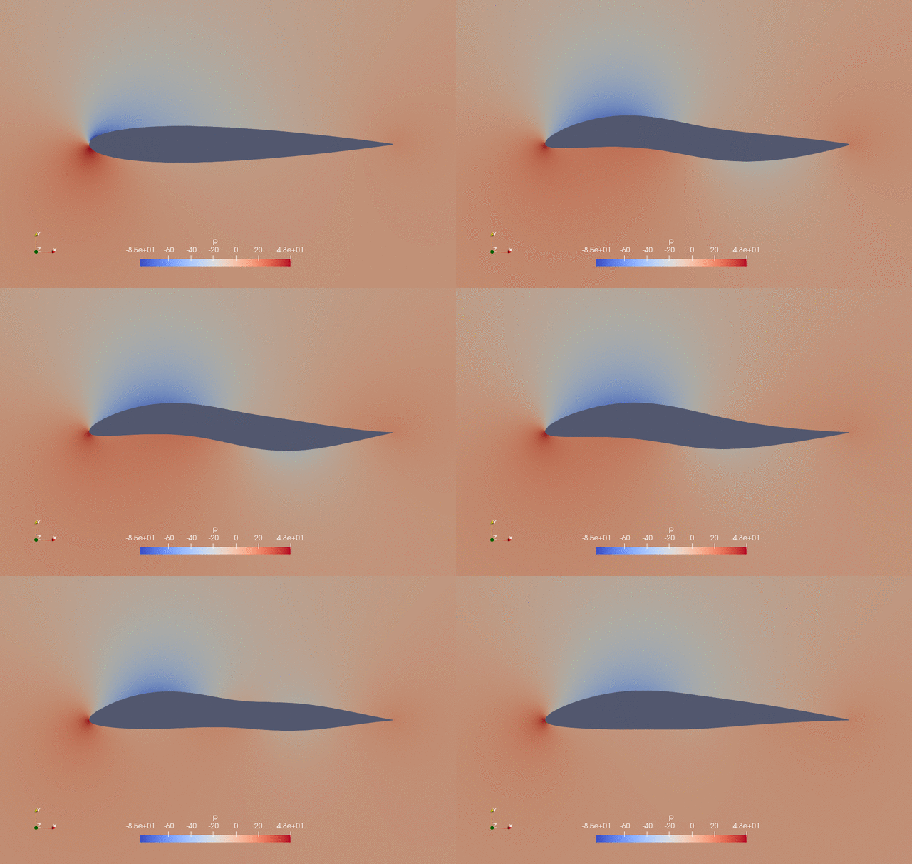
The case ran for 50 steps and took about 50 minutes using Intel 3.0 GHz CPU with 4 cores. According to logOpt.txt and opt_SLSQP.txt, the initial combined drag is 0.021973710 and the optimized drag is 0.017867543 with a drag reduction of 18.7%.
The evolution of pressure and shape during the optimization is as follows.

Fig. 2. Pressure and shape evolution during the optimization process